Abstract
Conditional diffusion models have the generative controllability by incorporating external conditions. However, their performance significantly degrades with noisy conditions, such as corrupted labels in the image generation or unreliable observations or states in the control policy generation. This paper introduces a robust learning framework to address extremely noisy conditions in conditional diffusion models. We empirically demonstrate that existing noise-robust methods fail when the noise level is high. To overcome this, we propose learning pseudo conditions as surrogates for clean conditions and refining pseudo ones progressively via the technique of temporal ensembling. Additionally, we develop a Reverse-time Diffusion Condition (RDC) technique, which diffuses pseudo conditions to reinforce the memorization effect and further facilitate the refinement of the pseudo conditions. Experimentally, our method achieves state-of-the-art performance across a range of noise levels on both class-conditional image generation and visuomotor policy generation tasks.
Method
Noisy conditions \(\tilde{y}\) entangle the clean conditional distribution \(p_0(x|y)\), producing a noisy conditional distribution \(p_0(x|\tilde{y})\). In this distribution, each noisy condition \(\tilde{y}\) can correspond to demonstrations from multiple clean conditions \(y\). This reduces feature consistency and makes vanilla conditional diffusion poorly controllable (Figure 1(b)). We correct noisy conditions by explicitly breaking this entanglement.Pseudo Condition (PC)
- Initialization: For each demonstration \( x_i \) in the noisy dataset, we initialize a pseudo condition \( \hat{y}_i \) as an all-zero vector of the same shape as \( \tilde{y}_i \), disrupting entangled clusters.
- Update: We update \( \hat{y} \) to approximate the clean condition \( y \) using temporal ensembling and early stopping. The update \( \hat{y}_{\phi} \) is predicted by a lightweight prediction head added to the diffusion model U-Net encoder (Figure 1(a)).
Reverse-Diffusion Condition (RDC)
- Augmentation: Inspired by the idea that diffusion training can be interpreted as data augmentation with Gaussian noise [2], we transfer the pseudo-condition \( \hat{y} \) into a diffusion process to augment its learning: \[ \left\{ \begin{aligned} &\text{Forward SDE:}~~ \mathrm{d}\hat{y} = \frac{-f(\hat{y}, t)}{g(t)} \mathrm{d}t + \frac{1}{g(t)} \mathrm{d}\mathbf{w}\text{,}\\ &\text{Reverse SDE:}~~ \mathrm{d}\hat{y} = \left( \frac{-f(\hat{y}, t)}{g(t)} - \frac{1}{g(t)^2} \nabla_{\hat{y}} \log p_t(\hat{y}) \right) \mathrm{d}t + \frac{1}{g(t)}\, \mathrm{d}\mathbf{\bar{w}} \text{,} \end{aligned} \right. \]
Image Generation Conditioned on Noisy Labels
We evaluated class-label image generation on noisy CIFAR-10 and CIFAR-100, using class labels as conditions and images as demonstrations.
We trained the baseline EDM and our method (PC+RDC) on the CIFAR-10 and CIFAR-100 datasets under symmetric noise (uniform mislabeling) with noise rates \( \eta \) = 20%, 40%, 60%, 80%. Table 1 shows that our method significantly surpass the baseline method EDM across all moderate and extreme noise level.
| Dataset | Noise Level | Method | FID (↓) | IS (↑) | Density (↑) | Coverage (↑) | CW-FID (↓) | CW-Density (↑) | CW-Coverage (↑) |
|---|---|---|---|---|---|---|---|---|---|
| CIFAR-10 | 0% | EDM | 1.92 | 10.03 | 103.08 | 81.90 | 10.23 | 102.63 | 81.57 |
| 20% | EDM | 2.00 | 9.91 | 100.03 | 81.13 | 16.21 | 88.45 | 77.80 | |
| Ours | 2.02 | 10.05 | 107.90 | 94.28 | 10.24 | 106.24 | 93.84 | ||
| 40% | EDM | 2.07 | 9.83 | 100.94 | 80.93 | 30.45 | 73.02 | 71.63 | |
| Ours | 2.17 | 10.04 | 105.88 | 93.80 | 10.64 | 102.96 | 93.18 | ||
| 60% | EDM | 3.67 | 9.70 | 99.14 | 83.99 | 51.69 | 53.47 | 74.12 | |
| Ours | 3.23 | 9.68 | 99.33 | 86.84 | 33.53 | 68.00 | 81.56 | ||
| 80% | EDM | 5.84 | 9.45 | 99.36 | 61.73 | 79.42 | 38.40 | 51.18 | |
| Ours | 4.25 | 9.58 | 103.53 | 78.73 | 68.39 | 47.35 | 56.70 | ||
| CIFAR-100 | 0% | EDM | 2.51 | 12.80 | 87.98 | 77.63 | 66.97 | 82.58 | 75.78 |
| 20% | EDM | 2.96 | 12.28 | 83.01 | 75.02 | 79.91 | 66.47 | 70.11 | |
| Ours | 3.18 | 12.95 | 98.32 | 93.52 | 71.57 | 90.49 | 91.51 | ||
| 40% | EDM | 3.36 | 11.86 | 81.70 | 73.92 | 100.04 | 49.77 | 60.64 | |
| Ours | 4.60 | 12.73 | 84.75 | 89.25 | 76.56 | 75.74 | 87.90 | ||
| 60% | EDM | 7.07 | 12.54 | 93.55 | 83.53 | 117.75 | 42.92 | 74.37 | |
| Ours | 5.57 | 12.03 | 91.89 | 87.45 | 104.34 | 67.39 | 84.03 | ||
| 80% | EDM | 11.13 | 12.66 | 92.09 | 71.53 | 146.97 | 25.02 | 52.57 | |
| Ours | 11.50 | 10.94 | 83.08 | 73.03 | 133.09 | 35.64 | 59.98 | ||
Figures 3 and 4 illustrate the generation processes of our model trained on CIFAR-10 and CIFAR-100 under 40% symmetric noise. To better visualize the robustness of our model trained with noisy condition, we fix the initial random noise of the demonstration and vary only the label condition. Taking Figure 3 as an example, each row corresponds to one class in the dataset. Each column shows the generation process under different class conditions starting from the same random noise, allowing a clear comparison of how the condition affects the generated image. It can be observed that, even under 40% noise, our method robustly generates images for all given classes.
Visuomotor Policy Generation Conditioned on Noisy Images
We conducted visuomotor policy generation experiments on the noisy Push-T dataset, where the task is to push a gray T-shaped block to a green target using image observations. Condition noise is simulated via radial (center magnification) and tangential (misalignment stretch) camera distortions, applied with probability \( \eta \) = 20%, 40%, 60%, 80% within preset intensities. As shown in Figure 5, we illustrate the differences between the original clean observations and the synthesized clean observations in the training set under 60% camera distortion.
Given these noisy Push-T datasets, we trained both the baseline Diffusion Policy (DP) and our method. After training, the policies generated by the DP model and our model were evaluated using Target Area Coverage (TAC), which measures the block-target IoU averaged over three seeds and 500 random initializations. As shown in Table 2, our method outperforms the baseline across all noise levels and demonstrates more stable performance.
| Noise Level | 20% | 40% | 60% | 80% |
|---|---|---|---|---|
| DP | 76.64 ± 1.67 | 73.02 ± 2.53 | 68.35 ± 5.00 | 68.46 ± 3.31 |
| Ours | 80.26 ± 1.07 | 73.44 ± 1.42 | 72.74 ± 1.21 | 71.78 ± 3.24 |
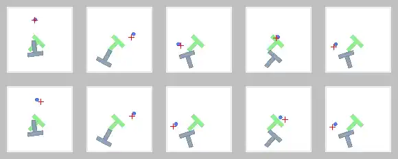
Figure 6 offers a clear visual comparison of policy generation between our method and the DP baseline. The first row displays policies from the baseline, and the second row shows those from our method, demonstrating that our method complete the pushing task more effectively.
Reference
- [1] Karras, T., Aittala, M., Aila, T., & Laine, S. (2022). Elucidating the design space of diffusion-based generative models. Advances in Neural Information Processing Systems, 35, 26565-26577.
- [2] Kingma, D., & Gao, R. (2023). Understanding diffusion objectives as the ELBO with simple data augmentation. Advances in Neural Information Processing Systems, 36, 65484-65516.
BibTeX
@article{chen2025robustlearningdiffusionmodels,
  title={Robust Learning of Diffusion Models with Extremely Noisy Conditions},
  author={Xin Chen, Gillian Dobbie, Xinyu Wang, Feng Liu, Di Wang, Jingfeng Zhang},
  journal={Arxiv},
  year={2025},
  url={https://arxiv.org/abs/2510.10149}
}